Total Annihilation has a special place in my heart since it was the very first RTS I played; it was with Command & Conquer and Starcraft one of the best RTS released in the late 90’s.

10 years later – in 2007 – its successor was released: Supreme Commander.
With Chris Taylor as the designer, Jonathan Mavor in charge of the engine programming and Jeremy Soule as the music composer (some of the main figures behind the original Total Annihilation), the expectations of the fans were very high.

Supreme Commander turned out to be highly praised by critics and players, with nice features like the “strategic zoom” or physically realistic ballistic.

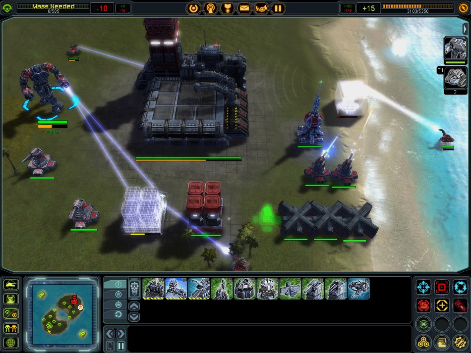
So let’s see how Moho, the engine powering SupCom, renders a frame of the game!
Since RenderDoc doesn’t support DirectX 9 games, reverse-engineering was done with the good old PIX.

Terrain Structure

Before we dig into the frame rendering, it’s important to first talk about how terrains are built in SupCom and which technique is used.

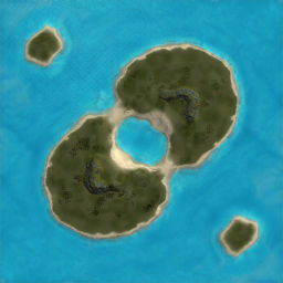
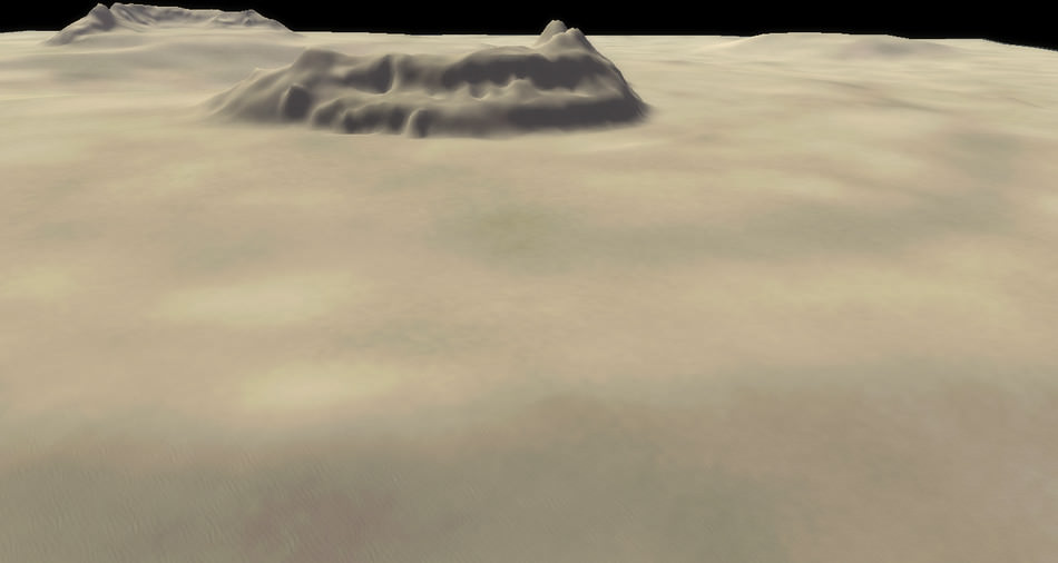
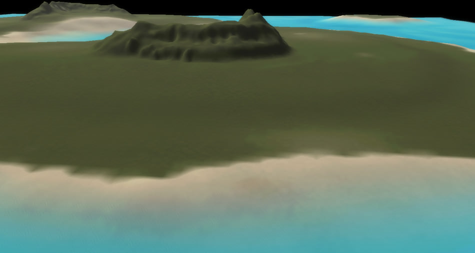
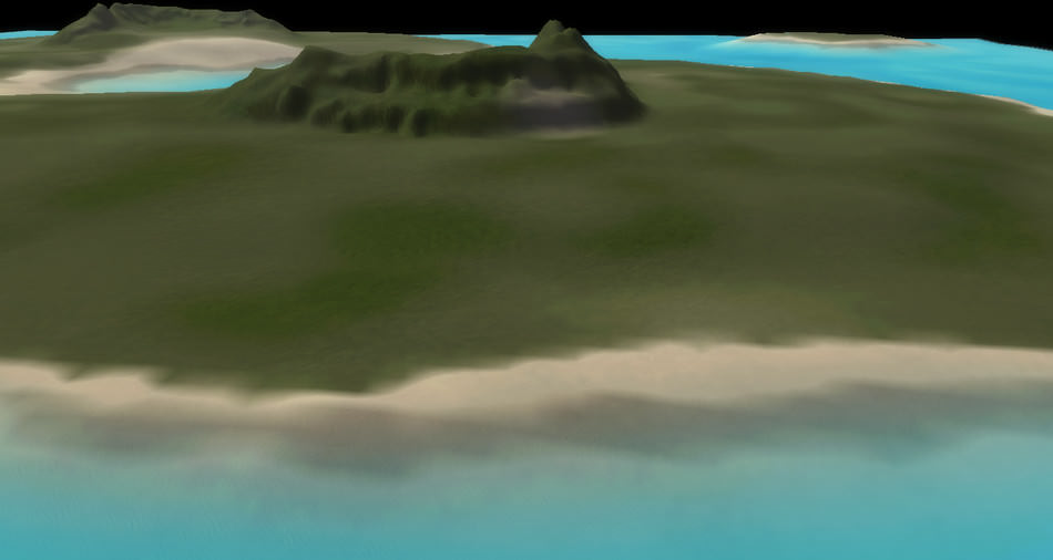
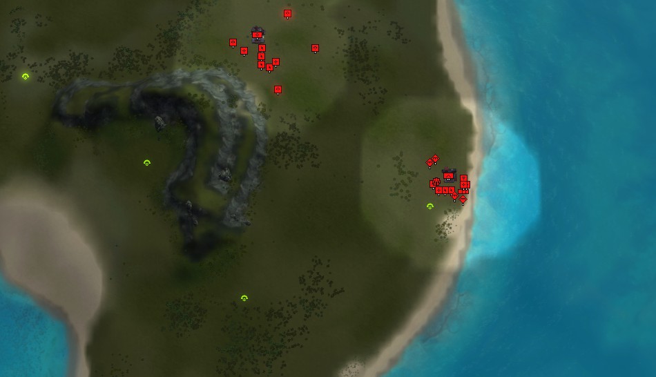
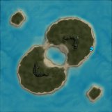
Here is an overview of “Finn’s Revenge”, a 1 versus 1 map.

On the left is a top-view of the entire map like it appears in-game on the mini-map.
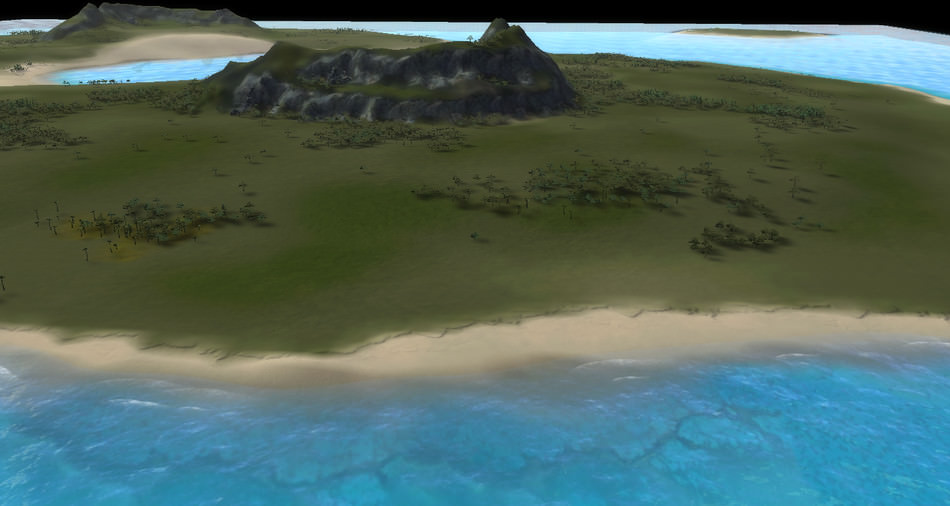
Below is the same map viewed from another angle:

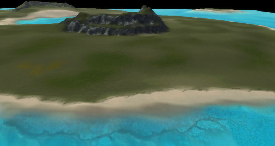
First the geometry of the terrain is calculated from an heightmap.
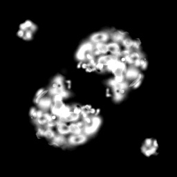
The heightmap describes the elevation of the terrain. A white color represents a high altitude and a dark one a low altitude.
For our map, a 513x513 single-channel image is used, it represents a terrain of 10x10 km in-game. SupCom supports much larger maps, up to 81x81 km.

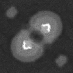
Heightmap

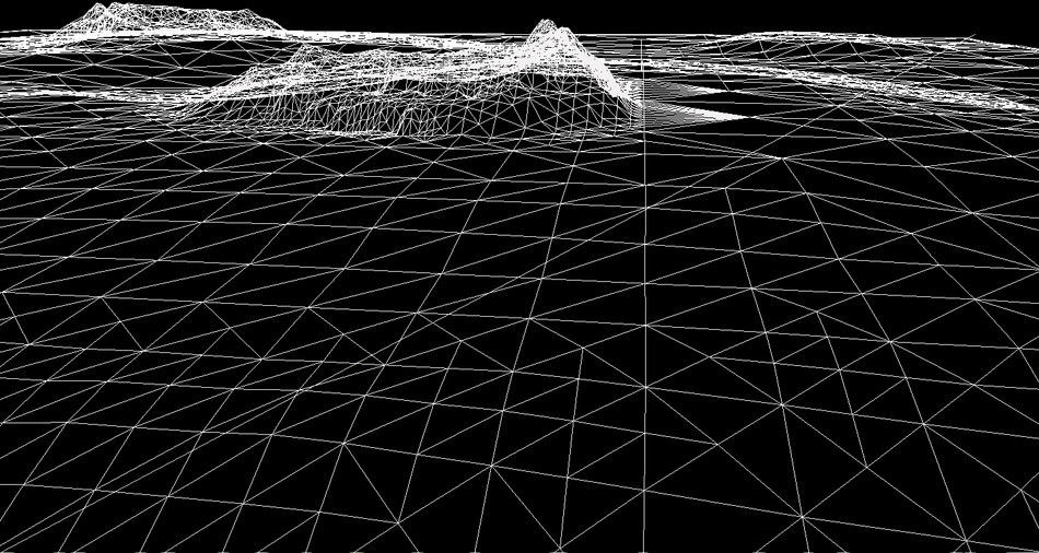
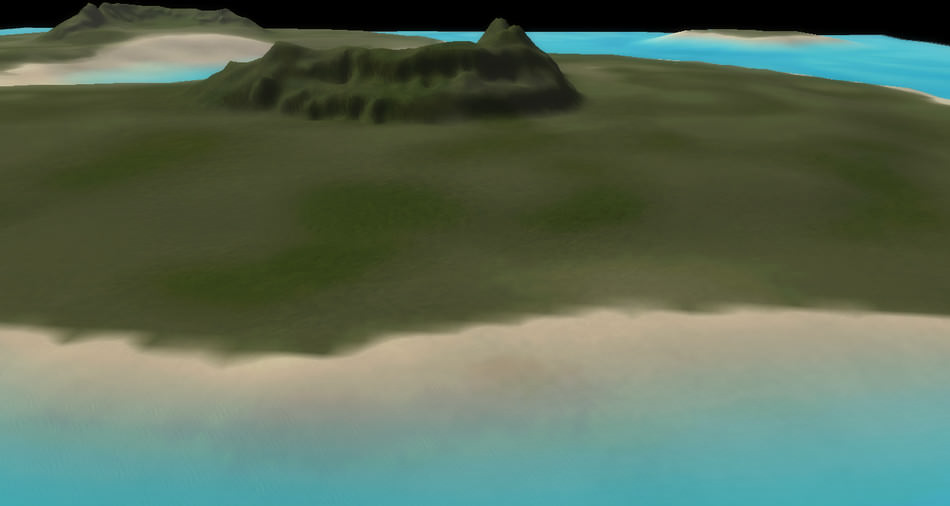
Tessellated Terrain

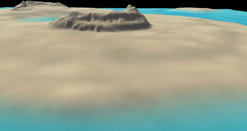
So we have a mesh which represents our terrain.
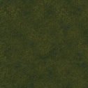
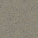
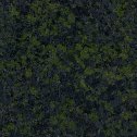
Then the game applies an albedo texture combined with a normal texture to cover all these polygons.
For each map the sea level is also specified so the game modulates the albedo color of the pixels under the sea surface to give them a blue tint.

Okay so having altitude-based texturing is nice, but it gets limiting quite quickly.
How do we add more details and variations to our map?

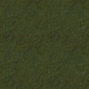
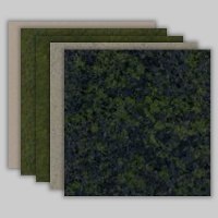
The technique used is called “Texture splatting”: the game draws a series of additional albedo+normal textures. Each step adds what’s called a “stratum” to the terrain.
We already have stratum 0: the terrain with its original albedo+color textures.
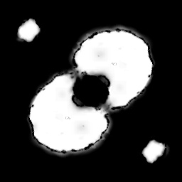
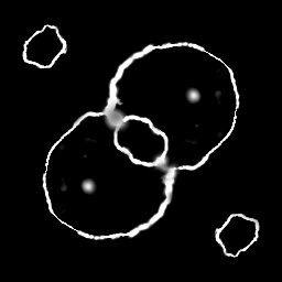
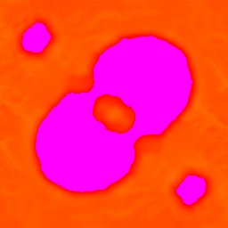
To apply the next stratum, we need some extra information: a “splat map”, to tell us where to draw the new albedo+normal and more importantly where not to draw! Without such a “splat map” also called alpha-map, applying a new stratum would completely cover the previous stratum. The albedo and normal textures both have their own scaling factor when they are applied to the mesh.

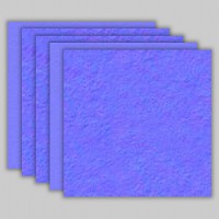
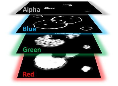
So we applied strata 1, 2, 3 and 4, each one relying on 3 separate textures. The albedo and normal textures use 3 channels (RGB) each, but the splat map uses only one channel.
So as an optimization the 4 splat maps are combined into a single RGBA texture.

Combined Splat Maps

Okay so we got more texture variations for our terrain. It looks nice from far away, but if you zoom-in you quickly notice the lack of high-frequency details.

This is when decals are applied: these are like small sprites which modify locally the albedo color and the normal of a pixel. This terrain has 861 instances of 21 unique decals.

It’s much better but what about some vegetation?
The next step is to add to the terrain what the engine calls “Props”: tree or rock models. For this map there are 6026 instances of 23 unique models.

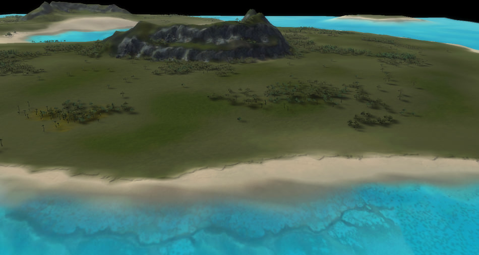
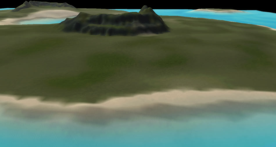
Now the final touch: the sea surface. It is a combination of several normal maps with UV scrolling along different directions, an environment map for reflections and sprites for the waves near the shores.

Our terrain is now ready.
Creating good heightmaps and splat maps can be challenging for map designers, but fortunately there are several tools to help with the task: there is the official “Supcom Map Editor” or World Machine with even more advanced features.

So now that we know the theory behind the SupCom terrains, let’s move on to an actual frame of the game.

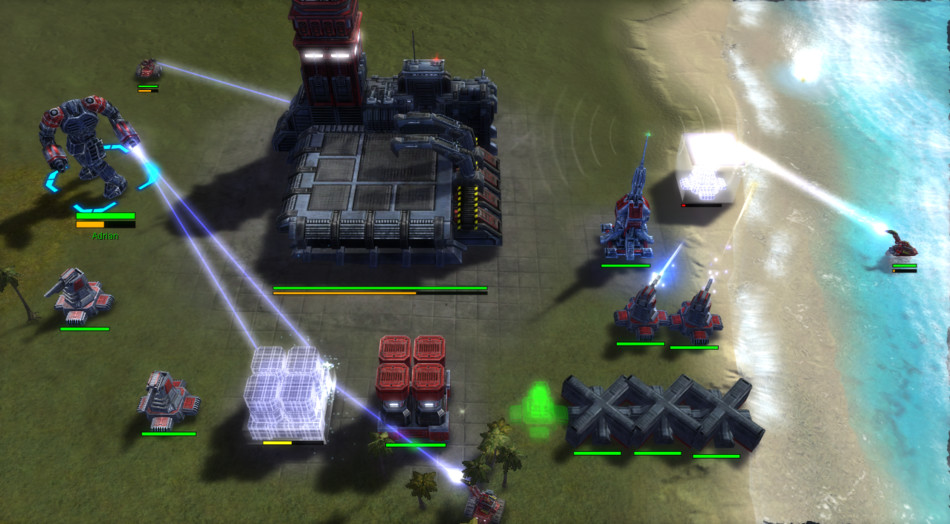
Frame Breakdown

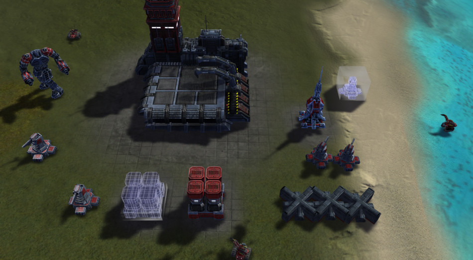
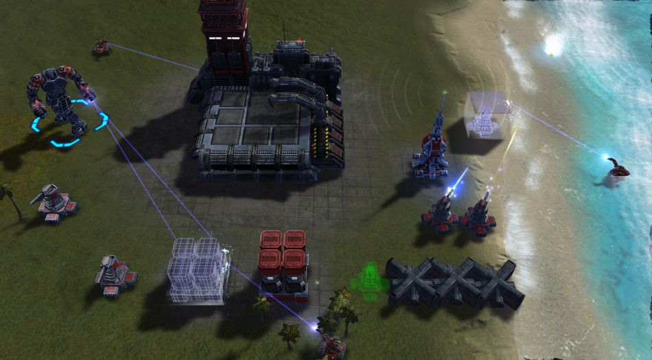
This is the game frame we’ll dissect:

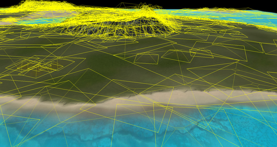
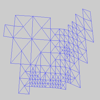
Frustum Culling

The game has in RAM the terrain mesh, created from the heightmap, it is tessellated by the CPU and the position of each vertex is known. When the zoom level changes, the CPU re-calculates the tessellation of the terrain.
Our camera focuses on a scene near the shore. Rendering the whole terrain would be a waste of calculation, so instead the engine extracts a submesh of the whole terrain, only the portion visible to the player, and feeds this small subset to the GPU for rendering.

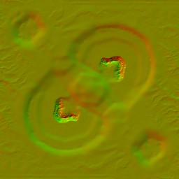
Normal Map

First, only the normals are calculated.
A first pass computes the normals resulting from the combination of the 5 stratums (5 normal maps and 4 splat maps).
The different normal maps are blended together, all the operations are done in tangent space.

Submesh Normals x5 Splatmaps

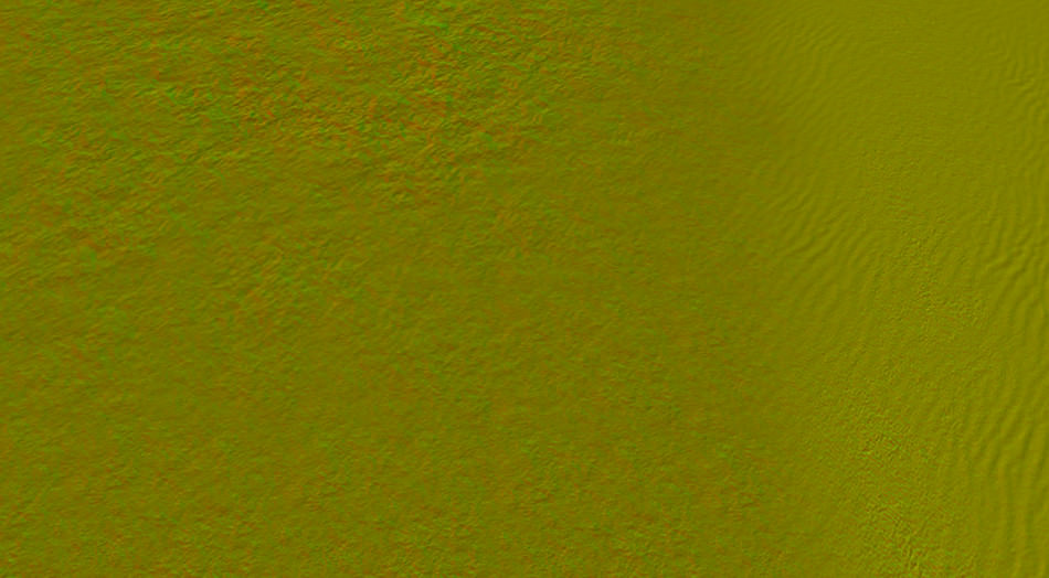
Normal Map

This is done in a single draw call with 6 texture fetches. You’ll notice the result is quite “yellowish”, it contrasts with the other normal maps which tend to be blue. And indeed: here the Blue channel is not used at all, only the Red and Green.
But wait, a normal is a 3-component vector, how can it be stored only with 2 components? It’s actually a compression technique (explained at the end of the post).
For now let’s just assume the Red and Green channels contain all the information we need about the normals.

Stratums are done, now it’s the turn of the decals: terrain decals and building decals are added to modulate the stratum normals.

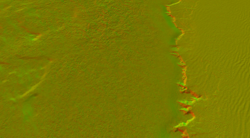
We still haven’t used the Blue and Alpha channels of our render target.
So the game reads from a 512x512 texture representing the whole normals of the terrain (baked from the original heightmap), and calculates for each pixel its normal using a bicubic interpolation. The results are stored in the Blue and Alpha channels.

Normal Map

Bicubic interpolation stored in Blue and Alpha.

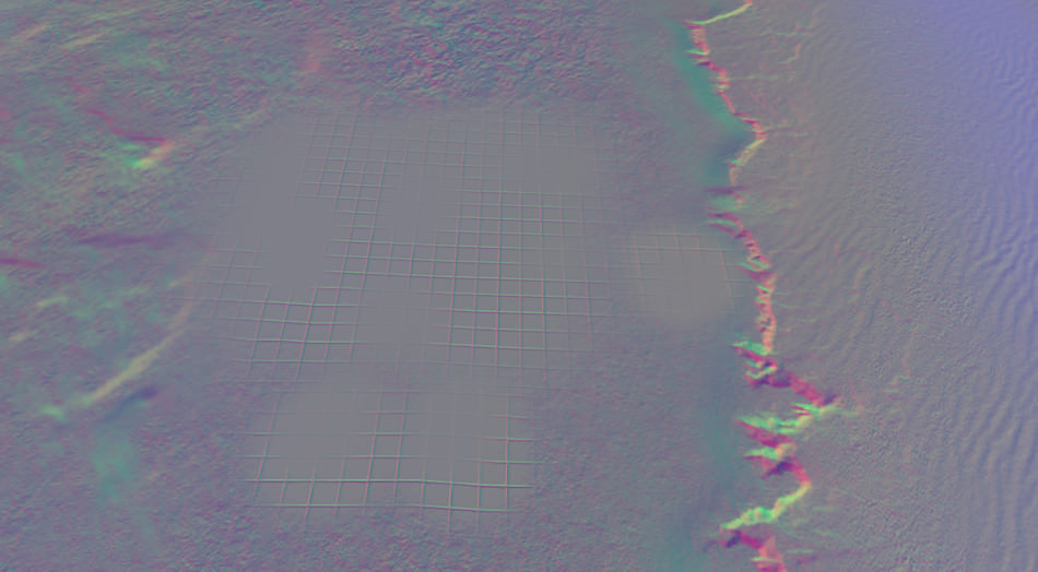
Red & Green: Stratum/Decal Normals Blue & Alpha: Base Terrain Normal

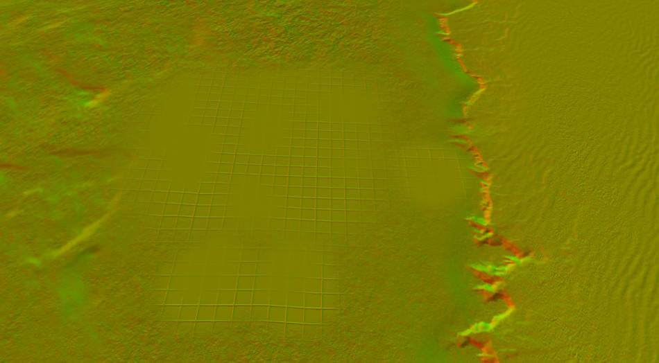
Then the game combines these two sets of normals (stratum/decal normals and terrain normals) into the final normals used to calculate the lighting.

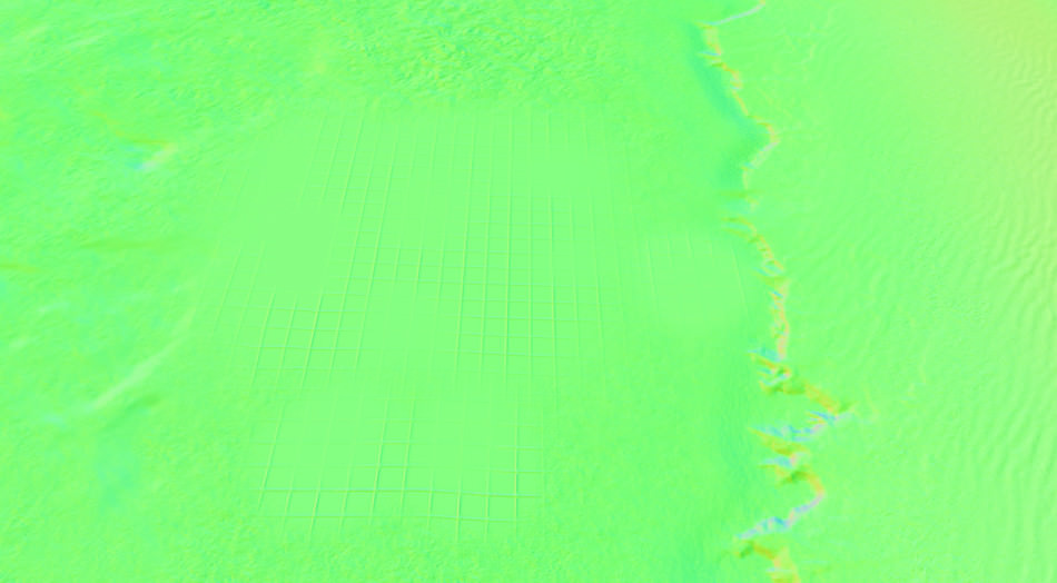
This time there’s no compression: the normals use the 3 RGB channels, one for each component.
It might look very green, but this is because the scene is quite flat, the result is correct: you can take any pixel and calculate its normal vector by doing colorRGB * 2.0 - 1.0, you can also check that the norm of the vector is 1.

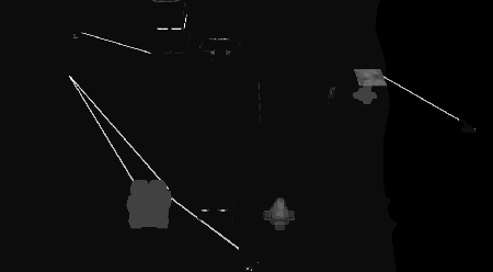
Shadow Map

The technique used to render the shadows is the “Light Space Perspective Shadow Maps” or LiSPSM technique.
Here we just have the sun as a directional light. Each mesh of the scene is rendered, and its distance from the sun is stored into the Red channel of a 1024x1024 texture. The LiSPSM technique calculates the best projection space to maximize the precision of the shadow map.

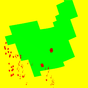
If we stop here, we would just be able to draw hard shadows. When the units are rendered, the game actually tries to smooth-out the edges of the shadows by using some PCF sampling.

But even with PCF, there would be no way to obtain the beautiful smooth-shadows we see on the screenshot, especially the smooth silhouettes of the buildings on the ground… So how was this achieved?

Even during the final parts of the development process of the game, it seems the implementation of shadows was still an on-going effort. This is what Jonathan Mavor was saying 11 months before the game public release:

The shadows in those shots are not finished and we do have a little bit of work to do on them yet. […]
We are not finished with the game graphically by any stretch at this point.

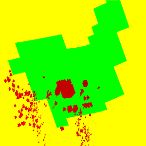
Just one month after this declaration, a new ground-breaking shadow map technique was emerging: Variance Shadow Maps or VSM. It was able to render gorgeous soft shadows very efficiently.
It seems the SupCom team tried to experiment with this new technique: decompiling the D3D bytecode reveals a reference to a DepthToVariancePS() function which computes a blur version of the shadow map. Before VSM was invented, shadow maps could not and were never blurred.
Here SupCom performs a 5x5 Gaussian blur (horizontal and vertical pass) of the shadow map.

LiSPSM

Gaussian Blur

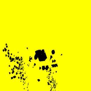
Blurred Shadow Map

However in the D3D bytecode, there is no instruction about storing the depth and the squared-depth (information required by the VSM technique). It seems to be only a partial implementation: maybe there was no time to perfect the technique during the final stages of the development, but anyway the code as-is can already produce nice results.

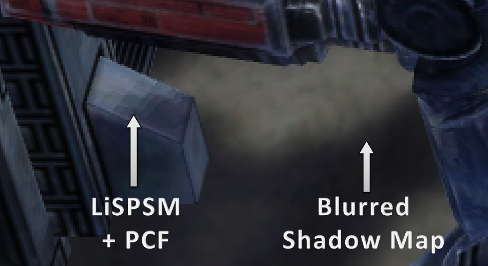
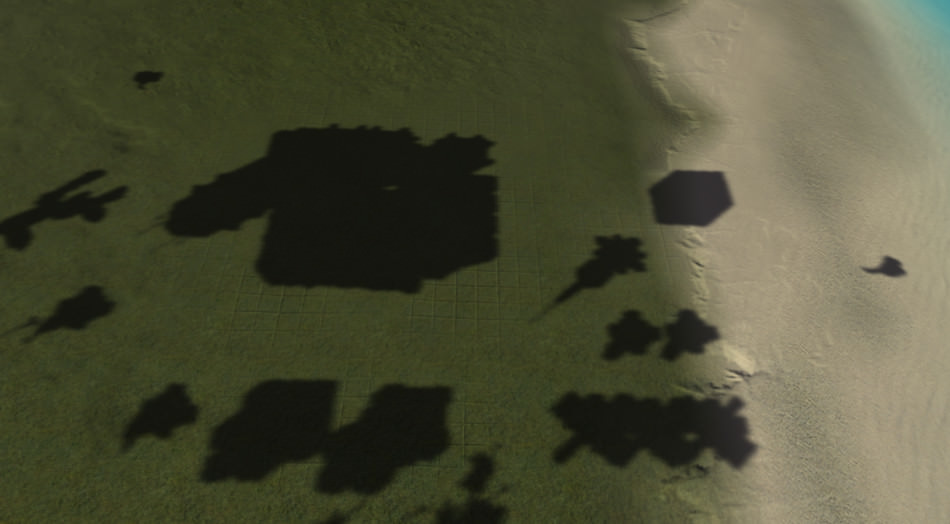
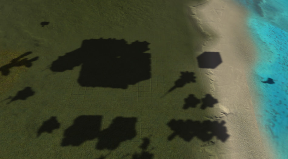
Note though that the pseudo-VSM map is used only to produce soft-shadows on the ground.
When a shadow must be drawn onto a unit, it is done through the LiSPSM map with PCF sampling. You can see the difference in the screenshot below (PCF has blocky artifacts at the shadow border):

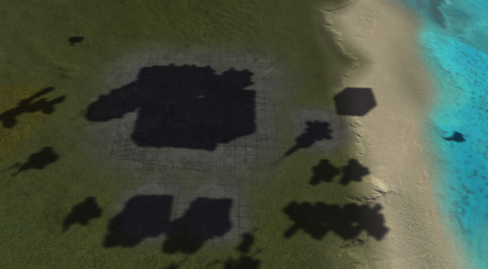
Shadowed Terrain

Thanks to the normal map and the shadow map that were generated, it is possible to finally start rendering the terrain: a textured mesh with lighting and shadows.

SplatMaps

Water Depth Map

Albedo Textures

Shadow

Normal

Decals

The albedo components of the decals are drawn, using the normal information to calculate the lighting equation.

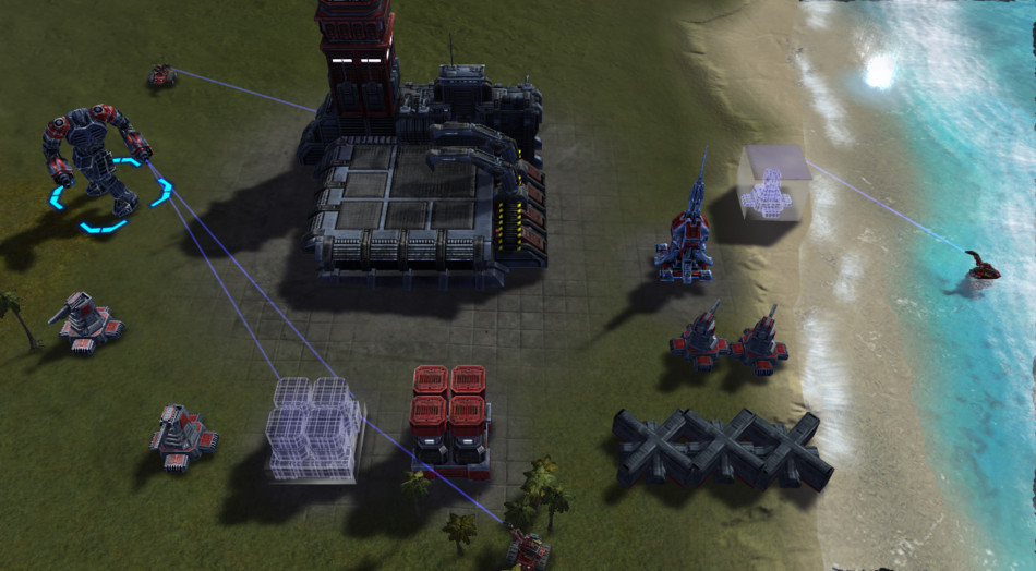
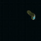
Water Reflection

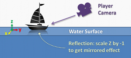
We have the sea on the right of our scene, so if a robot is sitting in the middle of the water we should be able to see its reflection on the sea surface.

A classic trick exists to render the reflection of a surface: an additional pass is performed, and just before applying the camera transformation, the vertical axis is scaled by -1 so the entire scene becomes symmetric with regards to the water surface (just like a mirror) which is exactly the transformation needed to render the reflection. SupCom uses this technique and renders all the mirrored unit meshes into a reflection map.

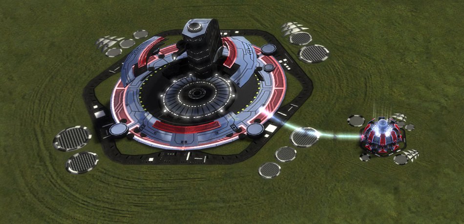
Mesh Rendering

All the units are then rendered one by one. For the vegetation, geometry instancing is used to render multiple trees in one draw call. The sea is rendered using a single quad, with a pixel shader fetching several normal maps, a refraction map (the scene rendered up until now), a reflection map (just generated above) and a skybox for additional reflection.

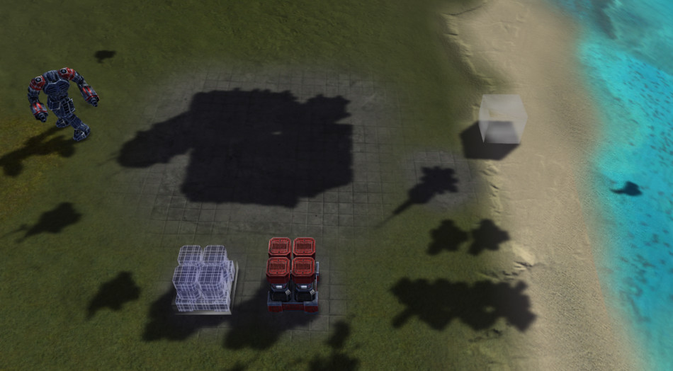
Notice in the last image the small black artifacts of the sea near the screen border: it’s because the sampling of the surface of the water is disrupted to create an illusion of movement. Sometimes the disruption brings texels from outside the viewport within the viewport: but such information does not exist, hence the black areas.
During the game the UI actually hides these artifacts under a thin border covering the edges of the viewport.

Mesh Structure

Each unit in SupCom is rendered in a single draw call. A model is defined by a set of textures:

• an albedo map
• a normal map
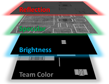
• a “specular map” which actually contains much more information than the specular. It’s an RGBA texture with:
  • Red: Reflection. How much the environment map is reflected.
  • Green: Specular. In regards to the sun light.
  • Blue: Brightness. Used later to control the bloom.
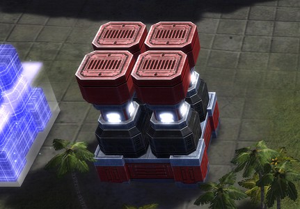
  • Alpha: Team Color. It modulates the unit albedo depending on the team color.

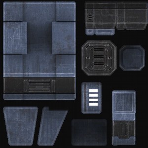
Albedo Map

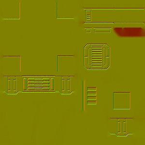
Normal Map

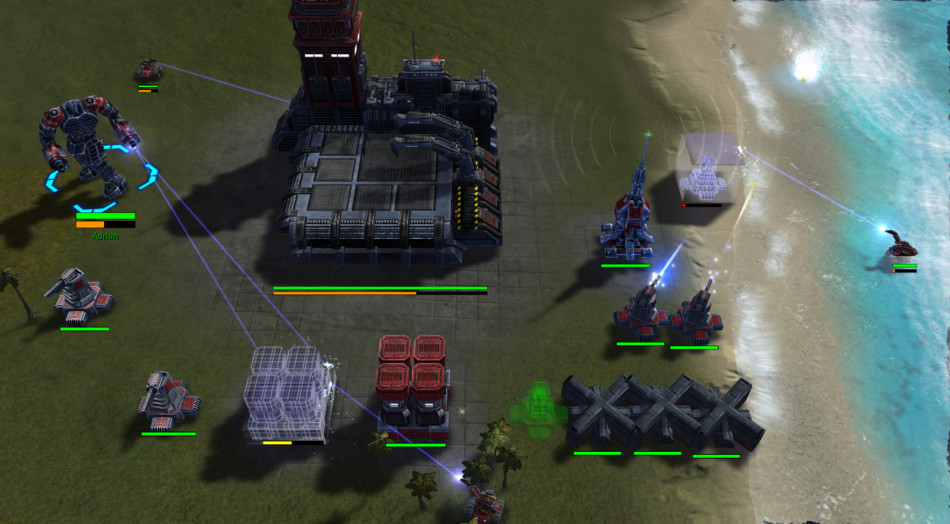
Particles

All the particles are then rendered and the health bars of each unit are also added.

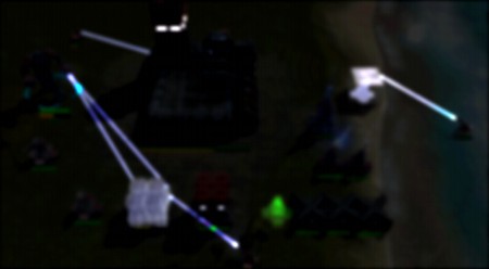
Bloom

Time to make things shine! But how do we get the “brightness information” since we’re working with LDR buffers?
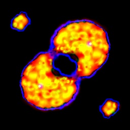
The brightness map is actually contained within the alpha channel, it was being built at the same time the previous meshes were drawn.
A downscaled copy of the frame is created, the alpha channel is used to make only the bright areas stand out and two successive Gaussian blurs are performed.

Alpha Channel

Brightness Blurred

The blurred buffer is then drawn on the top of the original scene with additive blending.

User Interface

We’re done concerning the main scene. The UI is finally rendered, and it is beautifully optimized: a single draw call to render the entire interface. 1158 triangles are pushed at once to the GPU.

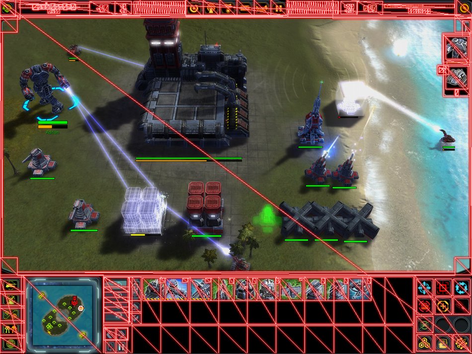
The pixel shader reads from a single 1024x1024 texture which acts like a texture atlas. When another unit is selected, the UI is modified, the texture atlas is regenerated on-the-fly to pack a new set of sprites.

And we’re done for the frame!

Additional Notes

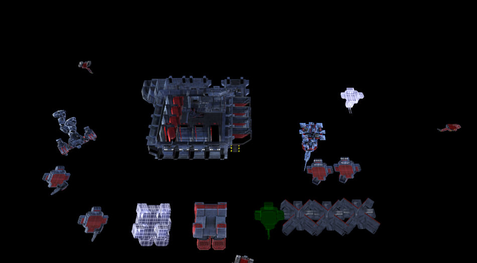
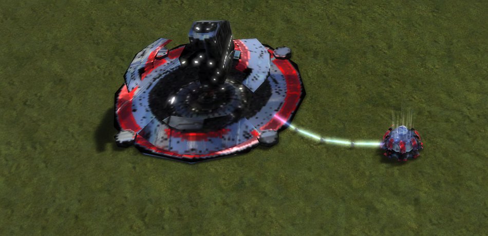
Level of Detail

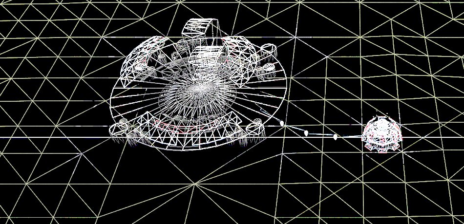
Since SupCom supports huge variations in the zoom level, it relies heavily on level of detail or LOD.
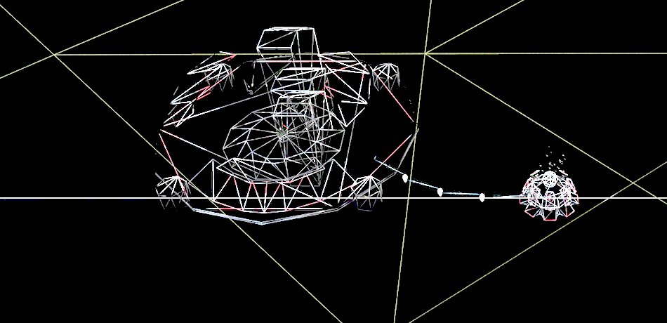
If the player zooms out from the map, the number of visible units quickly increases, to keep up with the increase in GPU load it becomes necessary to render simpler geometry and smaller textures. Since the units are very far away, the engine can get away with it: models are replaced with low-poly versions, with fewer details but they’re rendered so small on the screen that the player can hardly see the difference with high-poly models.

LOD does not only concern units: shadows, decals and props stop being rendered beyond a certain distance.

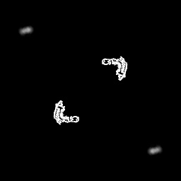
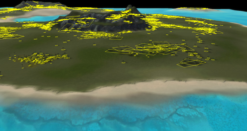
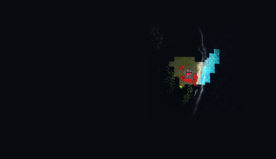
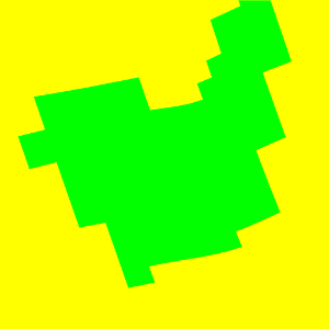
Fog of War

Because of the fog of war, each unit has a line of sight and only the area close to the units is completely visible. Areas where no units are present are either gray (previously visited) or black (still unexplored).
The game stores the fog information in a 128x128 mono-channel texture which defines the intensity of the fog: 1 means no visibility whereas 0 means full visibility.

Normal Compression

As promised, here is a short explanation about the trick used in SupCom to compress normals.
A normal is usually a 3-component vector, however in tangent space, the vector is expressed relatively to the surface tangent: X and Y are within the tangent plane while the Z component always points away from the surface.
By default the normal is (0, 0, 1) which is why most normal maps appear bluish when the normal is not perturbed.

So assuming the normal is a unit-vector, its length is one: X² + Y² + Z² = 1.
If you know the values of X and Y, then Z can only have two possible values: Z = ±√(1 - X² - Y²).
But since Z always points away from the surface, it has to be positive and so we have Z = √(1 - X² - Y²).
That’s why only storing X and Y in the Red and Green channels is enough, Z can be derived from them. A more detailed (and better) explanation can be found in this article.

Normal Blending

Since we are talking about normals, SupCom performs some kind of lerp between normal maps, using the splatmaps as factors. Actually there are several ways of blending two normal maps, with different results, it is not a straightforward problem like this article explains.

More Links

• The blog of Jonathan Mavor has a lot of technical insights and a very nice post about the TA Graphics Engine.
• The story behind TA development. Very interesting read from 1998, archived on the Wayback Machine.
• Details about SupCom map editing and modding.

More discussion on this very topic: Slashdot, Hacker News, Reddit.
Also, a print copy of this article has been made available by Hacker Monthly.